The Bellman $k$-segmentation algorithm generates a segmented constant-line
fit to a data series, but in trying to learn and implement this algorithm, I
found it difficult to find the segmentation algorithm rather than the
[apparently more common] $k$-means algorithm, so in this article I describe
and provide code for the $k$-segmentation algorithm.
Introduction
Richard Bellman is probably best known for his work on the Bellman–Ford algorithm (which generates the single-source shortest path on a weighted graph), but his biggest contribution to algorithms was the development of dynamic programming. In short, dynamic programming is applied to algorithms which need to solve a problem by considering smaller sub-problems, but these sub-problems are often repeated across many different cases. By using some extra memory to remember the answers to already-seen answers, the run-time can be vastly decreased.
The $k$-segmentation algorithm we want to describe is exactly one such
example of a dynamic programming problem. Before we can understand that this is
true, though, we need to define exactly what we want to achieve with this
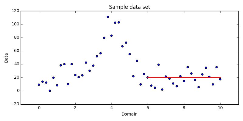
algorithm. Consider a series of $N$ data points, such as in Fig. 1.1.
The data would not be represented well by a single line, so the common
least-squares regression is insufficient. Instead, we might choose to model the
data using several constant line segments. For example, visually it is easy to
see that the data between about 6 and 10 could be approximated well by a line
segment passing through them along the x-axis.
In general, though, we can’t do this by hand for all data. Instead, we want a
way to quantify how well a fit models the given data and from that, determine
what the best set of line segments are to use. In more specific terms, we want
to determine a $k$ segments piece-wise constant regression (where $1\le k \le N$) of the $N$ data points. (In general, $k=1$ with a single degree of
freedom is a poor choice since it’s actually worse than the 2 degrees of
freedom least squares fit we already rejected, and $k=N$ doesn’t model the
data at all since a single line segment can be used for each data point.)
Formally, we’ll define the problem as:
This particular form of the error function is chosen for its applicability to dynamic programming solutions; you can see a much longer discussion showing this fact in my article on choosing a computationally efficient distance function.
Dynamic programming approach
Building from the ground up, there are two conditions we need to demonstrate
the $k$-segmentation problem meets before we can apply dynamic programming
techniques to the implementation:
Optimal substructure: The solution must rely on a subproblem being an optimal solution for the total solution to also be optimal.
Overlapping subproblems: The solutions method must share a small subset of common subproblems which are needed many times. In contrast, non-overlapping subproblems leads to the simpler divide-and-conquer paradigm.
Optimal substructure
For this problem, the most obvious way to demonstrate the optimal substructure
property is to consider successive values of $1 \le k' \le k$ through
induction to find an appropriate recursion relation.
Let the notation $E_S[i,k']$ represent the segmentation error over the data
points $\{x_1,\ldots,x_i\}$ using $k'$ segments, and let $E[i,j]$ be the
error in representing the points $\{x_i,\ldots,x_j\}$ using just the mean of
the data.
For the trivial case of $k' = 1$, we simply fit a single line segment as the
mean over all data points, with an associated error $E_S[N,1] = E[1,N]$.
Next, allow a second line segment to be used. The question becomes at which
point $i$ do we add the line segment so that there are two line segments from
$1...i$ and $(i+1)...N$. The error in this case is then
Moving up to $k' = 3$ is more complicated yet. Now when we append a line
segment to the end, we have two boundaries we need to determine. Instead of
thinking of the problem as finding two boundaries, though, we can take the
viewpoint that we’re still adding a segment to the end, but simply over a
longer sequence. (I presciently defined $E_S$ with this in mind since we can
specify where the end of the data sequence is.) In this light, let’s recast the
previous two cases in terms of “growing” sequences:
The extension to the case $k' = 3$ should now be obvious, so through
induction, let us skip straight to the generic recursion relation.
The optimal substructure in the problem is hopefully obvious in this form: in
order to know the optimal $k'$-segmentation solution, we need to know what
the optimal $(k'-1)$-segmentation solutions are. Because these are recursion
relations, storing the answer very rapidly saves computational time over
descending the recursion tree every time a particular answer is needed.
Overlapping subproblems
We can also very quickly demonstrate how the algorithm satisfies the
overlapping subsproblems property by inspecting Eq. $\ref{eqn:recurse}$.
The $E[j,i]$ term can be required many, many times for a particular choice of
$(j,i)$, and this by definition is an overlapping subproblem. Maybe less
obviously, the $E_S[j-1,k'-1]$ term also demonstrates the overlapping
subproblem property. If you remember to consider it in terms of a recursion
tree, the child subproblems (at the $k'-1$ level) will depend on overlapping
solutions at the grandchild ($k'-2$) level.
Algorithm design
Before continuing, you can download the IJulia notebook used to generate the sample data, analyze the data, and plot the figures. If you want to play around with the algorithms more, this notebook already contains a copy of the code we will be developing.
The rest of this article will deal with the details of the algorithm design to solve this problem. There are three major parts: pre-computing the error for subsequences with respect to their mean, calculating the segmentation errors, and reconstructing the solution. We’ll take each part in turn.
Subsequence errors
As required in the recursion relation we described in
Eq. $\ref{eqn:recurse}$, we need to know the error of representing any
arbitrary subsequence by its mean. For this purpose, we use distance function
described in
another article I’ve written
(which is very similar to the mean-squared error, differing in the overall
normalization and inclusion of a weighting term). For a detailed description,
see that article, but here we’re just concerned with the results:
The important part to note here is that the error is defined in terms of three
partial sums $W[i,j]$, $S[i,j]$, and $Q[i,j]$. These are useful because
as simple sums, any two arbitrary (disjoint) subsequences can be combined with
a three quick additions of the partial sums and then a recalculation of the
error term. In the other article, I show that a convenient choice of growing
longer subsequences is to just append each subsequence with the next element,
as graphically shown in Fig. 3.1. The red arrows point from the two terms
combined in each partial sum to generate the new longer subsequence partial
sums.
Another thing to note is that this is shown as a matrix. With our errors being defined in terms of indices of the beginning and ending of a subsequence, it is convenient (both visually and progmatically) to consider the indices as the row and column into a matrix. (In a similar manner, we’ll later build a non-square matrix for the total segmentation error.)
Now to dig into the code. Since we need the error over all subsequences for
every iteration of the recursion relation, it makes sence to precompute this
matrix, so we define a function prepare_ksegments which will produce the
errors. The only two inputs we need are the data series and a matching list
of weights:
function prepare_ksegments(series::Array{Float64,1}, weights::Array{Float64,1})
    N = length(series);
Next we initialize the partial sums and error matrices, but we do so by filling the diagonal immediately since it’s comprised of single element only data products. The error matrix is just generated as an empty matrix.
    wgts = diagm(weights);
    wsum = diagm(weights .* series);
    sqrs = diagm(weights .* series .* series);

    dists = zeros(Float64, N,N);
Hopefully the animated sequence in Figure 3.1 makes the form of the loops clear: we are going to proceed right-ward from the diagonal and as you go, there are less rows to move through on each iteration. The contents of the loop should be self-explanatory and just encapsulate the contents of the sums shown above.
    for δ=1:N
        for l=1:(N-δ)
            r = l + δ;

            wgts[l,r] = wgts[l,r-1] + wgts[r,r];
            wsum[l,r] = wsum[l,r-1] + wsum[r,r];
            sqrs[l,r] = sqrs[l,r-1] + sqrs[r,r];

            dists[l,r] = sqrs[l,r] - wsum[l,r]*wsum[l,r]/wgts[l,r];
        end
    end
Finally, we can note that everything we need to calculate the means of each subsequence is already being stored in the temporary partial sum matrices, and since we’ll need the mean values of particular subsequences later, we can precompute those as well. Inserting the appropriate matrix initialization and calculations for the means, the final function in total takes the form:
function prepare_ksegments(series::Array{Float64,1}, weights::Array{Float64,1})
    N = length(series);

    # Pre-allocate matrices
    wgts = diagm(weights);
    wsum = diagm(weights .* series);
    sqrs = diagm(weights .* series .* series);

    # Also initialize the outputs with sane defaults
    dists = zeros(Float64, N,N);
    means = diagm(series);

    # Fill the upper triangle of dists and means by performing up-right
    # diagonal sweeps through the matrices
    for δ=1:N
        for l=1:(N-δ)
            # l = left boundary, r = right boundary
            r = l + δ;

            # Incrementally update every partial sum
            wgts[l,r] = wgts[l,r-1] + wgts[r,r];
            wsum[l,r] = wsum[l,r-1] + wsum[r,r];
            sqrs[l,r] = sqrs[l,r-1] + sqrs[r,r];

            # Calculate the mean over the range
            means[l,r] = wsum[l,r] / wgts[l,r];
            # Then update the distance calculation. Normally this would have a term
            # of the form
            #   - wsum[l,r].^2 / wgts[l,r]
            # but one of the factors has already been calculated in the mean, so
            # just reuse that.
            dists[l,r] = sqrs[l,r] - means[l,r]*wsum[l,r];
        end
    end

    return (dists,means)
end
Segmentation errors
With the subsequence errors done, we can now work on calculating the
segmentation errors. As an implementation choice, I’ve done all of this work
directly in the regression interface regress_ksegments. The regression
interface again needs the data and weights, and it also to know how many
segments to fit to the data. We then immediately calculate and store the
subsequence errors.
function regress_ksegments(series::Array{Float64,1}, weights::Array{Float64,1}, k::Int)
    N = length(series);

    (one_seg_dist,one_seg_mean) = prepare_ksegments(series, weights);
Instead of a square look-up matrix for the subsequence error $E[i,j]$ as we
used in the previous section, the total segmentation error $E[i,k']$ is
stored in a non-square matrix. There are as many rows as possible values of
$k'$, but you’ll notice that instead of a width of $N$ for the number of
data points, I’ve added an extra column. This extra “ghost” column is logically
placed on the left to allow the algorithm to explore the possibility that the
best possible fit includes no previous segments and instead is best fit by a
single average over all elements.
At this point, the ghost column is already initialized (to zero) since we want
there to be no consequence for choosing to not use previous segments—in most
conceivable situations, the high cost of using a single subsequence average
will be disfavored due to the high cost. The other initialization we need is
for the case where $k'=1$. As we already showed, this is just the single
subsequence error, so we can copy that from $E[1,i]$.
    k_seg_dist = zeros(Float64, k, N+1);
    k_seg_path = zeros(Int, k, N);
    k_seg_dist[1,2:end] = one_seg_dist[1,:];
The k_seg_path variable we initialized is used at the end for reconstructing
the optimal solution. A common characteristic of dynamic programming problems
is that they also require some tracking information to solve the full problem.
Without this matrix, we could report the error of the optimal
$k$-segmentation regression, but we wouldn’t actually be able to show what
that regression is. The index into the matrix is the right (inclusive) boundary
of a segment, and the value it contains is the left (exclusive) boundary. This
means that the correct initialization for all $k'=1$ regressions stretch to
the beginning of the list. Likewise, if we use $N = k’$, then the left boundary
points to the previous elements. (The complicated syntax in the second line
below just indexes this “diagonal” in a single line of code.)
    k_seg_path[1,:] = 0;
    k_seg_path[sub2ind(size(k_seg_path),1:k,1:k)] = (1:k) - 1;
We make use of the fact that the recursion relation in
Eq. $\ref{eqn:recurse}$ can be transformed into a loop (also known as
tail recursion) and just start at $k'=2$ (remember, we initialized the first
case) and work our way up to $k'=k$. The inner loop runs over all possible
choices of the final subsequence length, and inside that, we just sum the
segmentation and single-subsequence errors. We then find the minimum total
error and record the location into the path reconstruction matrix and error
value into the total error matrix.
    for p=2:k
        for n=p:N
            choices = k_seg_dist[p-1, 1:n] + one_seg_dist[1:n, n]';

            (bestval,bestidx) = findmin(choices);
            k_seg_path[p,n] = bestidx - 1;
            k_seg_dist[p,n+1] = bestval;
        end
    end
At this point, we know the cost of the optimal solution (which is stored in
$E_S[N,k]$) but what we really want to know is what the optimal regression
is. The final bit of code does this by constructing a return array of length
$N$ with every data point set to its appropriate mean.
We start with the right-hand side pointing to the $N$-th element for the
solution with $k$ segments. The path matrix tells us where the left-hand side
of the optimal segment is to be located, so we fill in the regression values
over that segment with the appropriate mean. We then repeat for the $k-1$
remaining segments by moving up a row in the matrix and start with the
right-hand side to the immediate left of the just-generated segment.
    reg = zeros(Float64, size(series));

    rhs = length(reg);
    for p=k:-1:1
        lhs = k_seg_path[p,rhs];
        reg[lhs+1:rhs] = one_seg_mean[lhs+1,rhs];
        rhs = lhs;
    end
Putting all of these pieces together, along with some error checking and some convenience interfaces that let us forgo explicitly stating the weighting if we want uniform weighting, we have:
function regress_ksegments{T<:Number}(series::AbstractArray{T,1}, k::Int)
    # Fill in weights with default value if not given.
    weights = ones(Float64, size(series)) / length(series);

    return regress_ksegments(float(series),weights,k)
end

function regress_ksegments{T1<:Number,T2<:Number}(series::AbstractArray{T1,1}, weights::AbstractArray{T2,1}, k::Int)
    return regress_ksegments(float(series),float(weights),k)
end

function regress_ksegments(series::Array{Float64,1}, weights::Array{Float64,1}, k::Int)

    # Make sure we have a row vector to work with
    if (length(series) == 1)
        # Only a scalar value
        error("series must have length > 1")
    end

    # Ensure series and weights have the same size
    if (size(series) != size(weights))
        error("series and weights must have the same shape")
    end

    # Make sure the choice of k makes sense
    if (k < 1 || k > length(series))
        error("k must be in the range 1 to length(series)")
    end

    N = length(series);

    # Get pre-computed distances and means for single-segment spans over any
    # arbitrary subsequence series(i:j). The costs for these subsequences will
    # be used *many* times over, so a huge computational factor is saved by
    # just storing these ahead of time.
    (one_seg_dist,one_seg_mean) = prepare_ksegments(series, weights);

    # Keep a matrix of the total segmentation costs for any p-segmentation of
    # a subsequence series[1:n] where 1<=p<=k and 1<=n<=N. The extra column at
    # the beginning is an effective zero-th row which allows us to index to
    # the case that a (k-1)-segmentation is actually disfavored to the
    # whole-segment average.
    k_seg_dist = zeros(Float64, k, N+1);
    # Also store a pointer structure which will allow reconstruction of the
    # regression which matches. (Without this information, we'd only have the
    # cost of the regression.)
    k_seg_path = zeros(Int, k, N);

    # Initialize the case k=1 directly from the pre-computed distances
    k_seg_dist[1,2:end] = one_seg_dist[1,:];

    # Any path with only a single segment has a right (non-inclusive) boundary
    # at the zeroth element.
    k_seg_path[1,:] = 0;
    # Then for p segments through p elements, the right boundary for the (p-1)
    # case must obviously be (p-1).
    k_seg_path[sub2ind(size(k_seg_path),1:k,1:k)] = (1:k) - 1;

    # Now go through all remaining subcases 1 < p <= k
    for p=2:k
        # Update the substructure as successively longer subsequences are
        # considered.
        for n=p:N
            # Enumerate the choices and pick the best one. Encodes the recursion
            # for even the case where j=1 by adding an extra boundary column on the
            # left side of k_seg_dist. The j-1 indexing is then correct without
            # subtracting by one since the real values need a plus one correction.
            choices = k_seg_dist[p-1, 1:n] + one_seg_dist[1:n, n]';

            (bestval,bestidx) = findmin(choices);

            # Store the sub-problem solution. For the path, store where the (p-1)
            # case's right boundary is located.
            k_seg_path[p,n] = bestidx - 1;
            # Then remember to offset the distance information due to the boundary
            # (ghost) cells in the first column.
            k_seg_dist[p,n+1] = bestval;
        end
    end

    # Eventual complete regression
    reg = zeros(Float64, size(series));

    # Now use the solution information to reconstruct the optimal regression.
    # Fill in each segment reg(i:j) in pieces, starting from the end where the
    # solution is known.
    rhs = length(reg);
    for p=k:-1:1
        # Get the corresponding previous boundary
        lhs = k_seg_path[p,rhs];

        # The pair (lhs,rhs] is now a half-open interval, so set it appropriately
        reg[lhs+1:rhs] = one_seg_mean[lhs+1,rhs];

        # Update the right edge pointer
        rhs = lhs;
    end

    return reg
end
Example regressions
Using the same data as shown in the introduction, we can now apply a
$k$-segmentation regression on the data. Here I’ve chosen to show how the
regression changes under two choices of the weighting. The first case is for
uniform weighting, shown in Fig. 4.1.
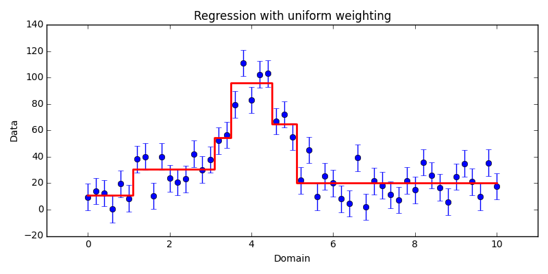
$k$-segmentation regression applied to our sample data set using uniform
weighting. Here, the uniform weight factor was chosen to be 10 simply for
visualization purposes; the default weight factor would have instead chosen
0.0196 corresponding to $1 / N$.The second case shows the affect of weighting the data non-uniformly. The
particular weighting choice corresponds to statistical counting error
estimate—if the value of a particular bin is $I$, we expect the error on the
counts to be $\sqrt{I}$ and correspondingly choose a weight which is the
reciprocal square error ($1/I$). In this case we see that the segments are
pulled to different locations because the low-error data points incur a larger
regression error if they are not fit well than the points with large error.
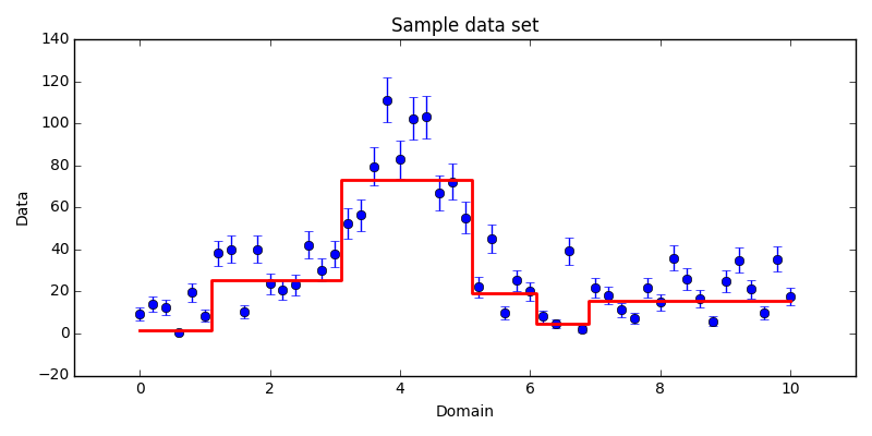
$k$-segmentation regression applied to our sample data set using counting
statistics error and weight estimates on each data point. The regression
appropriately changes to minimize the regression error incurred.- Niina Haiminen, Aristides Gionis, & Kari Laasonen. “Algorithms for unimodal segmentation with applications to unimodality detection.” Knowledge and Information Systems, 2008, Vol.14(1), pp.39-57 DOI: 10.1007/s10115-006-0053-3