One of the simplest statistical properties of a data set is its mean. The next step is often to quantify how well the mean represents the data. A variety of techniques exists, but in this article, I show why the mean-squared error is an excellent choice for dynamic programming algorithms. The mean-squared error has the advantage that it coincides well with our intuitive idea of distance (being closely related to Euclidean distance) as well admitting a computationally efficient implementation.
Motivation
I was originally motivated to investigate efficient ways of calculating the distance function described in the next section while implementing a dynamic programming problem. The salient detail of any dynamic programming problem is that they are designed to accelerate computations by reusing of answers from already-computed sub-problems. Mathematically, this is often expressed as a recursion relation aligning with the optimal substructure of the problem.
For example, in the context of fitting data to a model, the best overall fit
occurs when subsets also obtain an optimal fit. If $g(i,j)$ is the goodness
of fit for a model over data points $i$ through $j$ and $c(k)$ is the
cost for combining two fits at point $k$, then the recursion relation could
take the form
A performance gain is realized when the recursion relation is used to build
from a previous answer rather than naively calculating the goodness of fit over
all $j$ elements each time (the naive implementation giving
$\mathcal{O}(N^3)$ performance, assuming constant computational time per data
point). If instead the recursive approach above can be performed using stored
knowledge—and it can, as will be demonstrated—the expense of the calculation is
greatly reduced (to $\mathcal{O}(N^2)$ for the same assumptions).
Defining the problem
Let $\{x_i\}$ be a set of $N$ ordered data points with associated weight
$\{w_i\}$ with $w_i > 0$. Further, denote the weighted mean of the data by
$\bar x$.
We then want to define a distance function $d[x]$ which quantitatively
evaluates how well the data $\{x\}$ is represented by the single mean value
$\bar x$. A good fit should be indicated by a smaller number while poor fits
will have increasingly large distances.
Euclidean distance function
The Euclidean distance is a natural starting point for a cost function since it coincides with our physical intution about distances. The Pythagorean theorem is taught in the context of a 2D plane, so only two values are summed in quadrature to give the hypoteneuse across a triangle. In 3D, the sum of squares includes three terms which gives the distance across opposite corners of a rectangular prism.
The Euclidean distance is just the natural extension to an arbitrary number of dimensions by summing the terms in quadrature.
Weighted error distance function
Rather than finding the distance across $N$ dimensions, though, we want to
find the distance between data points and their mean, or the “error distance”.
Abstractly, this is not a different problem since there are still $N$ degrees
of freedom. The only change we make is that we are summing the squares of the
errors $\{e_i\}$ rather than the values of the data points themselves.
Another extension we want to introduce at this point is how to handle the uncertainty in a measurement. Data points which are known more precisely should affect the distance more strongly just as is done in the weighted average. In a form similar to the weighted average (Eq. \ref{eqn:weighted}), we simply weight each error value by the weights (and maintain normalization by dividing by the sum of the weights).
At this point we’ve just rederived the weighted variance, but we need to
start simplifying to get a computationally useful result. First, the square
root is a problem if we wish to manipulate the distance function into a form
which resembles the recursion relation in Eq. $\ref{eqn:recurse}$.
Thankfully we can apply any monotonic transformation to the function and the
ordering of distances will be maintained. In this case, the transformation is
obvious—raising to an even power is a monotonic transformation, so we can
simply square $d[x]$.
Second, the denominator was added to maintain normalization, but as a sum of
terms, it can never be factored to allow separation of terms. Again, though,
removing it is a monotonic transformation (multiplying by a constant), so we
can eliminate it with no consequence. This leaves us with our distance function
$\mathcal{D}[x]$.
Factoring the distance function
To permit us to incrementally update the distance function, we start by
expanding the terms of $\mathcal{D}[x]$ and explicitly insert the definition
of $\bar x$.
To see how terms can be separated from one another, we can choose to fully
separate the $i=1$ term from the rest and expand $j=1$.
Then by grouping similar terms,
we eliminate a factor of the denominator in the last term and note that the second and third terms are then the same form. Therefore, we simplify to
Now make the identifications
and the explicit, expanded form of $\mathcal{D}[x]$ can be rewritten as
Each of these three terms are completely separable and can be updated on the fly for any set of data points. We didn’t identify a way to directly produce a distance function with this property, but we can easily generate the distance by keeping track of these three quantities and calculating the distance function as needed.
In the context of the dynamic programming problem, then, we calculate
$g(1,j)$ as a summation of the distance from two sub-sequences:
Example in dynamic programming
If you take note of the second distance function term in
Eq. \ref{eqn:dist_recurse}, you’ll see that the distance over all
possible pairs of $(k,j)$ will eventually need to be known. If we store
the answer (or more accurately, precompute the quantities and perform an
appropriate lookup as needed) we can avoid wasting computational resources
calculating the distance function for each pair of $(k,j)$ every time.
In this case where we’re working with pairs of coordinates, it’s natural to
think of and store the data in a matrix. We’ll choose to use the upper
triangular portion of the matrix so that $k$ index the row and $j$ indexes
the column, consistent with matrix notation.
Generically, let us refer to any of the three quantities $w_i$, $w_i x_i$
and $w_i{x_i}^2$ by $z_i$, and use the shortcut notation $\sum_i^j \equiv \sum_{k=i}^j z_k$. As an initial condition, we need to define $z_i$ for each
of the quantities. These are then placed along the diagonal of the matrix as
shown in Fig. 6.1.

$[i,i]$ into the matrix
is simply the identity of a single element.Considering the formula we derived in Eq. $\ref{eqn:dist_split}$, a
longer subsequence’s value is calculated by summing two constituent
subsequences’ values. If you’re feeling particularly creative, there are many
ways to choose the subsequences, but the two most obvious are to either append
just one additional element at the beginning or the end of the list for each
subsequence. Here I have [arbitrarily] chosen to build each subsequence from
back to front.
What I want to do now is add the preceeding $z_i$ to the subsequence that
follows it if it does not already include the first element. Pictorially, this
means we start filling in the first off-diagonal by shifting the subsequence
up a row and pulling in (adding) the value from the diagonal. For the first
diagonal, this looks like Fig. 6.2.
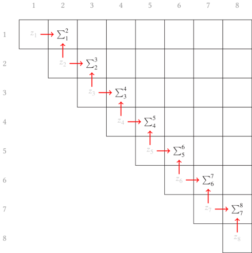
By induction, we continue this process until the entire upper triangular matrix has been filled with the information we seek. The sweep upward along the off-diagonals is animated in Fig. 6.3.
This process can be done in parallel for each of the $W$, $S$, and $Q$
functions/matrices defined in
Eqs. $\ref{eqn:weights}–\ref{eqn:squares}$. Then the distance matrix can
be computed (either by updating the corresponding element of $\mathcal{D}$
last in each loop iteration in a serial environment or as a post-condition in a
multithreaded environment).
I asserted in the introduction that the motivation for using a dynamic
programming approach to calculating costs could lead to an order
$\mathcal{O}(N^2)$ algorithm. It should be clear from this diagram that this
is true. (Remember that constants have no effect in asymptotic notation, and
since there are $\approx N^2/2$ elements being filled in each matrix with
just 4 matrices to create—the three partial sums and the final distance
matrix—we have pretty effectively demonstrated its expected performance just by
drawing out the dependency graph.)