An extremely common operation on data series is to regress the data with a particular model. Many times, the desired model is a linear combination of known basis functions, and when this is true, the regression of a data series can be encapsulated as a matrix operator. Describing the process as a matrix operation—rather than just using the regression coefficients—isn’t always useful, but it’s description is rarer. Because I needed a regression in this form for my research, I have chosen to write up the solution here.
Motivation
In my research, there’s a case when we regress and subtract a polynomial from some time stream data as a method of removing unwanted noise—a so-called polynomial filter. Such filtering is quite simple with most analysis software since regression functions are ready-made to return the fit polynomial, which can then just be subtracted from the data.
What happens, though, if—by design of the experiment—we know that the data will have particular length and data rate (i.e. the “x” values will all be the same), but we want to hold off on actually regressing the data until a later step? In my case, we want to describe how to apply analogous filtering to a simulation which won’t be generated until later.
The question, then, is if the filtering operation is linear so that we can simply encapsulate the operation as a matrix-vector multiplication where the matrix contains all the information necessary to apply the filtering upon the data vector. Whether you have experience to know that this is in fact true or not, we can start from just a couple of assumptions and derive an expression which constructs such a matrix.
Derivation
Various definitions of “best-fitting” model exist, but we’re going to choose
the common least-squares definition. To begin, let our data series ${(x_i, v_i)}$ be denoted by the vectors $x$ and $v$. (I’m going to forego adding
the arrows to vectors since we’ll very shortly write everything in terms of
matrix expressions where they’re unnecessary.) Our goal is to find a model
vector $m$ which minimizes the error $\chi^2$ in the chi-squared sense.
In matrix notation, the $\chi^2$ error is given by the expression
and the goal is to choose the best model $m_* = \{m | \min(\chi^2)\}$ which
minimizes the chi-squared error. Valid models are ones which are linear
combinations of some given set of basis functions; explicitly,
where $\varphi$ are the basis functions and $a$ are parameters which choose how
strongly each function contributes to the model. This vector $a$ is then the
free parameters which we are trying to choose correctly in order to construct
the best-fit model. We simply convert the above expression to matrix notation
by noting that it is just a series of two dot products:
Note that the choice to write $(\varphi x^\top)^\top a$ instead of naively writing
$x \varphi^\top a$ is to make it clear what the “operators” $\varphi$ actually operate
upon — for example, the order of terms if $\varphi = \partial/\partial x$ is important.
Because of this somewhat awkward notation, it is helpful to define the
regressor matrix $M \equiv (\varphi x^\top)^\top$ so that the model simply becomes
Plugging this into the definition of $\chi^2$, we determine the $a_*$
corresponding to $m_*$ by finding a minimum with respect to $a$.
The $v^\top v$ term is independent of $a^\top$ and therefore goes to
zero. Furthermore, the second term is a scalar, so we can transpose it to make
it identical to the third term without changing the value. We then have two
terms, one linear and one quadratic in $a^\top$, so performing the
differentation gives,
Therefore, we can conclude that you can in fact construct a matrix which captures a linear regression model according to
for $v$ a vector of length $n$ and $\varphi$ being a vector of $k$ linearly independent basis functions.
Numerical computation
In terms of mathematical theory, the formulation in Eq. $\ref{eqn:invfit}$ is probably sufficient and probably more practical to work with directly. Computationally, though, the matrix inversion creates problems. The issue is that matrix inversion algorithms are quite sensitive to the limitations of finite representations of floating point numbers and numerical instabilities.
The answer to these problems are to consider matrix decompositions (also called matrix factorizations). There are a very wide number of possible decompositions, but a common one because of its tendency to stabilize calculations is the orthogonal-triangular decomposition, also more commonly referred to as the QR decomposition. The QR decomposition is defined as
This is a particularly fruitful decomposition, as we’ll see. Start by applying
QR decomposition to the regressor matrix $M = QR$ so that the linear
regression becomes
where for $n$ data points in a $k$ parameter model, $M$ will be $n×k$, and $Q$
and $R$ will decompose as $n×n$ and $n×k$ matrices, respectively. By definition
of orthonormality, $Q^\top Q = QQ^\top = I$ where $I$ is the identity
matrix, so the middle multiplication term disappears.
If you know your linear algebra well, it might be clear that the middle
products of $R$s looks tantalizingly close to an identity that we know
results in the identity matrix—if not, see Appendix A
for a quick derivation. There is a problem, though: for that identity to hold,
the matrix $R$ must itself be invertible, and since it is not square, we
can’t define an inverse (ignoring the distinction that right- and left-inverses
can sometimes be defined).
We can keep simplifying, though, by noting a particularly special property
about $R$; by construction, it is an upper triangular matrix, and therefore
most of $R$ is filled with zeros. To be more specific, the upper triangle in
$R$ can be contained in a $k×k$ matrix, so we define
where $R_1$ is a $k×k$ matrix and the rest of the $(n-k)×k$ terms are
zeros. Likewise, we can create a corresponding split in $Q$, motivated by the
fact that many columns in $Q$ will only ever multiply the zero portion of
$R$. Let
so that
Note that $Q_1$ is no longer an orthonormal matrix; the additional columns of
$Q$ are critical to producing the orthonormality property that we imposed as
an assumption, but the product $QR$ can be perfectly represented by this
so-called reduced QR decomposition $Q_1 R_1$.
The special thing about this particular decomposition now is that, together
with the fact that we know $QR = Q_1 R_1$, we can rewrite the regression as
Since $R_1$ is square, we can finally invoke the matrix identity in
Appendix A and simplify this to
The particularly important part of this simplification is that we’ve managed to completely remove the matrix inversion step. Since the matrix inversion is the step that we worried most would lead to numerical instability, removing it entirely from the expression helps greatly in providing numerically accurate and stable regressions.
Application
Julia makes coding this analysis very simple since QR decomposition functions are built in to the standard library. These are actually just convenient wrappers around LAPACK, though, so similar algorithms can be developed for any language which can interface with LAPACK’s C/Fortran interface.
As always, an associated IPython notebook can be downloaded which includes the code and figures shown here.
Regression Interface
For the purposes of code reuse, it make sense to encapsulate the regression itself in reusable functions that take an arbitrary regressor matrix. Below I provide two such functions. The first returns a matrix which can be used to produce a regression over any input data which shares the same regressor matrix. The second is just a convenience wrapper which immediately applies the regression to a given data series.
# regress(R) -> F
#
# Takes in a regressor matrix R and returns a matrix which, when multiplied
# with a data vector, produces the regression.
#
function regress{T<:FloatingPoint}(R::Matrix{T})
    (q,r) = qr(R, thin=true);
    return q*q';
end

# regress(R, y) -> m
#
# Takes a regressor matrix R and applies the specified regression to y
# to return the model fit m.
#
function regress{T<:FloatingPoint}(R::Matrix{T}, y::Vector{T})
    return regress(R)*y;
end
Polynomial regression
The case in my research is application of polynomial filters. There are various choices of basis functions to describe polynomials (in particular, see the computationally expensive Chebyshev polynomials which are useful for interpolation), but the simplest is the one everyone is familiar with from high school algebra: the powers of $x$.
Note that the monomials do not produce an orthogonal basis, but nowhere did we require that. (In many cases, though, orthogonal basis functions are useful since mathematicians and physicists have gone through great efforts to enumerate their properties for other purposes.)
# polyregressor(n, x) -> R
#
# Produces a regressor matrix for an n-th order polynomial at the given
# x positions suitable for use with regress().
#
function polyregressor{T<:FloatingPoint}(n::Integer, x::Vector{T})
    N = length(x);
    R = Array(T, N, n+1);
    R[:,1] = one(T);
    for ii=2:n+1
        R[:,ii] = R[:,ii-1] .* x;
    end
    return R;
end
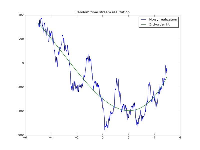
Regressing a data series is as simple as multiplying it against the resultant
matrix. In Fig. 4.1, I show a randomly generated time-stream using a
Gaussian random number stream $\{r_i\}$ sent through a first-order
auto-regressive model $y_i = y_{i-1} + r_i$ where $y_1 = r_1$ and then the
entire series is vertically shifted so that a random point in the series is
the zero crossing.
It is important to note again that the regression isn’t limited to polynomials — it is merely the case I was considering. Building regressors and applying them for exponentials, trigonometric functions, and logarithms are also easily performed.
Regression filtering
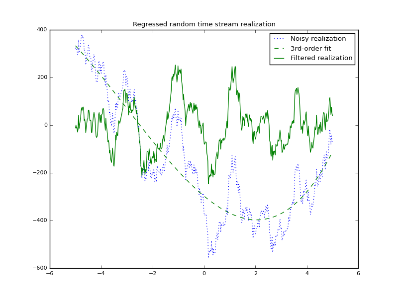
In some cases, it can be trivial to extend this work to cover new cases. For example, we can filter a time stream so that it no longer contains a third-order polynomial component. Once we realize that what we’re asking is for the residual above beyond the third-order fit,
then factoring out the $y$ by implicitly multiplying by the identity, we can identify a new filtering matrix $F$ that will perform—e.g. third-order polynomial—filtering of any input data.
Generic functions which perform this filtering operation are almost trivial to write since they simply extend the $regress$ functions we’ve already written.
# filt(R) -> F
#
# Takes in a regressor matrix R and returns a matrix which, when multiplied
# with a data vector, filters out the regression from the data.
#
function filt{T<:FloatingPoint}(R::Matrix{T})
    (q,r) = qr(R, thin=true);
    return eye(size(R,1)) - q*q';
end

# filt(R, y) -> m
#
# Takes a regressor matrix R and applies the specified filtering to the
# input data sequence.
#
function filt{T<:FloatingPoint}(R::Matrix{T}, y::Vector{T})
    return filt(R)*y;
end
Applying this filtering to the same data as presented in Fig. 4.1, we see the higher “modes” of the data plotted in Fig. 4.2.
Numerical tests
I stated that matrix inversion creates numerical instabilities that are best avoided by making use of matrix decompositions. This claim is easy enough to test empirically given the framework we’ve now created. The methodology is to generate a known function exactly, and then regress that data—first with a fit that makes use of matrix inversion, and a second time that uses the simplified QR decomposition case. Since by design there is no noise in the input data, any differences between the fit and regressions are due to numerical limitations of the algorithm used.
We’ll take a 3rd order polynomial as our test function, defined as
Then performing regressions using both schemes below, we plot the residual
$\delta_1$ as “matrix inversion method” and $\delta_2$ as “QR decomposition method”.
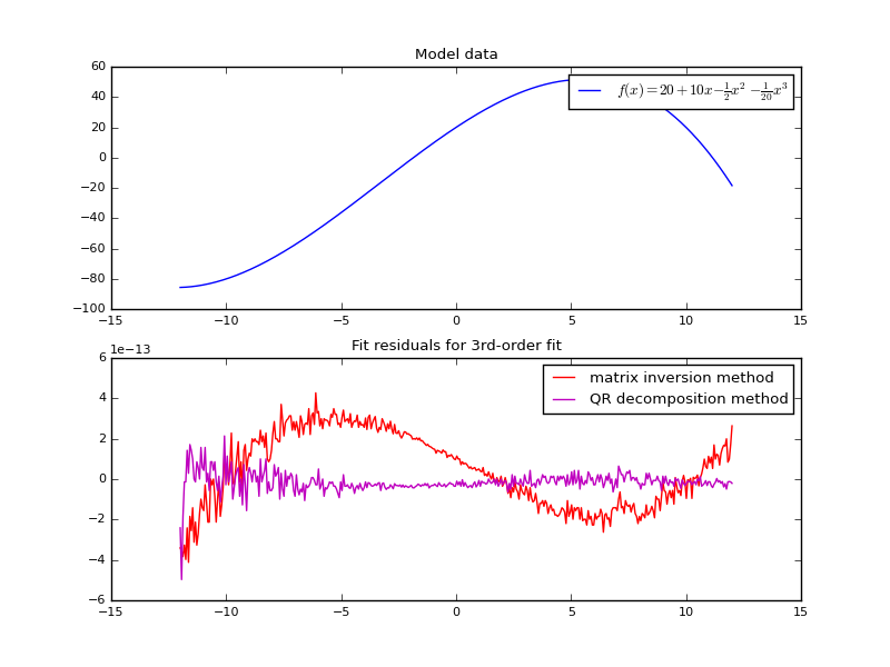
$f(x)$ using a third-order regressor
with two different solution algorithms. The matrix inversion method uses
explicit inversion of products of the regressor matrix, while the QR
decomposition method uses an approach that skips any need for matrix inversions
by conducting a convenient matrix decomposition.If we instead change the regressor to be a 6th order fit (still for a 3rd) order polynomial, we really start to see how quickly the numerical stability issues begin to plague the calculation.
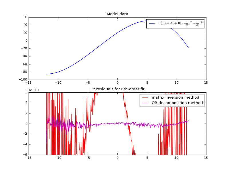
$f(x)$ using a sixth-order regressor
with two different solution algorithms. In comparison to Fig. 5.1, the
residuals in the matrix inversion method increase greatly, while very little
apparently changes in the QR decomposition method.Matrix product and inverse identity
We invoked an identity in Section 3 which allowed us to simplify a rather complicated looking matrix product to the identity. It’s not too difficult to derive from scratch, though, so we do that explicitly here.
Begin by assuming that we have some invertible, square matrix $A$. Then we
can construct a square, symmetric matrix $S$ by multiplying $A$ with its
own transpose.
The inverse of $S$ can then be described explicitly in terms of $A$ by
Next, left multiply $S^{-1}$ by $A$,
and then right multiply by $A^\top$,
Finally, by substituting back in the definition of $S$, we have proven our
desired identity. (Because of the symmetry of $A^\top A = A A^\top$, there’s
a second identity which is true, provable with only trivial changes to the
proof already written here.)