Building a color theme around a primary photo can be useful, but picking the “main” colors by hand can be a challenge. Thankfully using a couple of simple analysis techniques, we can extract a color palette automatically.
Introduction
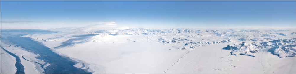
While designing this website, I needed an initial color palette to design the site theme around. One of the first choices I made was to select the header banner image — a panorama of the Antarctic Plateau I took on my flight from McMurdo Station to Amundsen-Scott South Pole Station in November 2016. Because the image is mostly dominated by shades of blue and gray, I thought it would work well to numerically extract the “typical” colors from the image.
We can load the image for analysis by using the Images.jl package.
using Images

img = load(download("https://justinwillmert.com/img/antarctic_plateau.jpg"))

1000×4001 Array{RGB{N0f8},2} with eltype RGB{Normed{UInt8,8}}:
 RGB{N0f8}(0.373,0.588,0.812)  …  RGB{N0f8}(0.408,0.569,0.773)
 RGB{N0f8}(0.373,0.588,0.812)     RGB{N0f8}(0.4,0.561,0.765)
 RGB{N0f8}(0.373,0.588,0.812)     RGB{N0f8}(0.408,0.565,0.769)
 RGB{N0f8}(0.376,0.58,0.808)      RGB{N0f8}(0.416,0.569,0.784)
 RGB{N0f8}(0.376,0.58,0.808)      RGB{N0f8}(0.412,0.565,0.78)
 RGB{N0f8}(0.38,0.576,0.808)   …  RGB{N0f8}(0.4,0.561,0.773)
 RGB{N0f8}(0.384,0.58,0.812)      RGB{N0f8}(0.4,0.569,0.776)
 RGB{N0f8}(0.384,0.58,0.812)      RGB{N0f8}(0.4,0.58,0.784)
 RGB{N0f8}(0.384,0.58,0.812)      RGB{N0f8}(0.404,0.573,0.78)
 RGB{N0f8}(0.38,0.584,0.812)      RGB{N0f8}(0.404,0.573,0.78)
 RGB{N0f8}(0.38,0.584,0.812)   …  RGB{N0f8}(0.404,0.573,0.78)
 RGB{N0f8}(0.38,0.584,0.812)      RGB{N0f8}(0.404,0.573,0.78)
 RGB{N0f8}(0.38,0.584,0.812)      RGB{N0f8}(0.408,0.576,0.784)
 ⋮                             ⋱  ⋮
 RGB{N0f8}(0.588,0.604,0.651)     RGB{N0f8}(0.686,0.698,0.733)
 RGB{N0f8}(0.592,0.608,0.655)     RGB{N0f8}(0.69,0.702,0.737)
 RGB{N0f8}(0.6,0.616,0.663)    …  RGB{N0f8}(0.686,0.698,0.733)
 RGB{N0f8}(0.6,0.616,0.663)       RGB{N0f8}(0.675,0.686,0.722)
 RGB{N0f8}(0.584,0.6,0.647)       RGB{N0f8}(0.702,0.702,0.733)
 RGB{N0f8}(0.596,0.612,0.659)     RGB{N0f8}(0.714,0.714,0.745)
 RGB{N0f8}(0.596,0.612,0.659)     RGB{N0f8}(0.706,0.706,0.737)
 RGB{N0f8}(0.592,0.608,0.655)  …  RGB{N0f8}(0.718,0.718,0.749)
 RGB{N0f8}(0.6,0.616,0.663)       RGB{N0f8}(0.714,0.714,0.745)
 RGB{N0f8}(0.6,0.616,0.663)       RGB{N0f8}(0.698,0.698,0.729)
 RGB{N0f8}(0.596,0.612,0.659)     RGB{N0f8}(0.714,0.714,0.745)
 RGB{N0f8}(0.592,0.608,0.655)     RGB{N0f8}(0.714,0.714,0.745)
The image img is a 2D array of pixel values where each pixel is a data
structure describing the colors of the pixel which act as a scalar value.
To do further calculations, we’ll want to view the pixels as vectors in
a color space.
The Colors.jl
package provides the necessary color space and representation conversions.
In particular, channelview reinterprets each pixel color value as a
vector in the given color space.
The image is an sRGB image, so each pixel is a 3-vector of normalized
intensities of the red, green, and blue channels:
using Colors

pix = channelview(reshape(img, :))
3×4001000 reinterpret(N0f8, ::Array{RGB{N0f8},2}):
 0.373  0.373  0.373  0.376  0.376  …  0.718  0.714  0.698  0.714  0.714
 0.588  0.588  0.588  0.58   0.58      0.718  0.714  0.698  0.714  0.714
 0.812  0.812  0.812  0.808  0.808     0.749  0.745  0.729  0.745  0.745
Once viewed as color vectors, we can easily perform any number of linear algebra calculation of choice. For example, the inner product between two pixels may be a useful metric to quantify how “close” the colors are to one another.
using LinearAlgebra: ⋅, normalize

p₁ = normalize(pix[:,1])
@show p₁ ⋅ p₁;
p₁ ⋅ p₁ = 1.0022774f0
The limits of the default data types — 8-bit normalized pixel values
(the RGB{N0f8} above) and conversion to 32-bit floating point during
operations — results in poor numerical accuracy of the subsequent
calculations.
Before continuing, we’ll want to convert the image to 64-bit floating point
values.
pix′ = channelview(convert.(RGB{Float64}, vec(img)))
p₁ = normalize(pix′[:,1])
@show p₁ ⋅ p₁;
p₁ ⋅ p₁ = 0.9999999999999999
Clustering
To calculate color clusters, we’ll use \(k\)-means clustering, which is closely
related to the
Bellman \(k\)-segmentation algorithm
I have previously written about.
Rather than using a generalization of that algorithm, we’ll make use
of the community’s
Clustering.jl
package.
using Clustering
The package provides a very simple interface for calculating clusters — choose
a number of clusters \(n\) and call kmeans. The return structure’s centers
field contains the coordinates of the \(n\) cluster centers.
using Random: seed!

n = 5
# control the initial conditions to have reproducible results
km = kmeans(pix′, n, init=floor.(Int, range(1, size(pix′,2), length=n)))
km.centers
3×5 Array{Float64,2}:
 0.23481   0.627798  0.421534  0.891051  0.801239
 0.40308   0.714616  0.603809  0.89823   0.814712
 0.551106  0.80912   0.790103  0.920897  0.849644
Reinterpreting each column as a normalized color vector gives us the generated color palette.
palette = colorview(RGB{Float64}, km.centers)

Finally, one last thing we can do with the km data structure is view the
original image recolored according to the clustered color palette.
The cluster struct contains the list of which cluster center each input
has been assigned to, so we can replicate the color palette according to
those assignments and reshape the vector back into the same shape as the
input image:
rc_pix = palette[assignments(km)]
recolored = reshape(rc_pix, size(img))

display(img)
display(recolored)
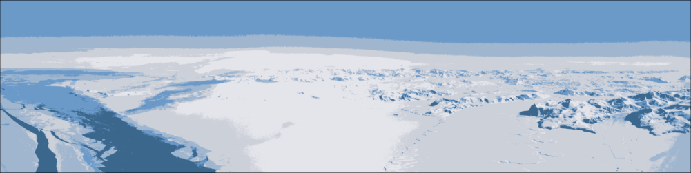
This view of the color palette makes it much clearer where each of the colors have been sourced from. As one would expect, the large swaths of snow and ice are clustered as various shades of grey, and the water and sky contribute blues.
Unfortunately, using only 5 colors in the palette means the clustering has lost much of the detail in the mountains near the center where the clouds and ice are too similar in color.
To make iterating on the number of colors easier, let us encode the entire palettizing process into a function:
function palettize(::Type{T}, imgin, n; seed=1111) where {T<:Color}
    @assert isconcretetype(T)
    img = convert.(T, vec(imgin))
    nimg = length(img)

    # Use initial points from the image rather than reseeding
    km = kmeans(channelview(img), n,
        init=floor.(Int, range(1, nimg, length=n)))

    pal = collect(colorview(T, km.centers));
    idximg = pal[assignments(km)]
    permute!(pal, sortperm(counts(km), rev=true))

    return (; palette=pal, recolored_img=reshape(idximg, size(imgin)))
end
palettize (generic function with 1 method)
Now let us preview what it’d look like to add two more color swatches to the palette:
palette7, recolored7 = palettize(RGB{Float64}, img, 7)
display(palette7)
display(recolored7)

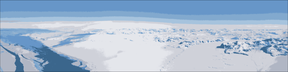
Freely allowing additional cluster items hasn’t helped very much to retain the details in the mountain peaks. Instead the sky has an additional band of color spanning the color gradient, and the very right edge of the image is a darker grey rather than a shade of blue.
Inspecting the original image, it’s natural to think that there should be
a section of nearly pure white which isn’t being automatically selected.
We can bias the clustering to include arbitrary colors by using a weighted
\(k\)-means clustering.
When no weights are provided, the implicit weighting is uniform, so to bias the result we need only provide a dummy pixel value for each desired color with a weight suffiently high to be a cluster center.
As an ansatz, we’ll take the forced colors to have a weight of unity before
renormalizing, which is approximately \(N_\mathrm{pix}\) times greater than
the standard weights of \(N_\mathrm{pix}^{-1}\) each.
# Initialize pixels and weights
img_wwhite = convert.(RGB{Float64}, vec(img))
w_wwhite = fill(1/length(img_wwhite), length(img_wwhite))

# Push a white pixel into the image with a high weight
push!(img_wwhite, colorant"white")
push!(w_wwhite, 1.0)
# renormalize: N*inv(N) + 1 == 2, so divide by 2
w_wwhite ./= 2; @assert sum(w_wwhite) == 1
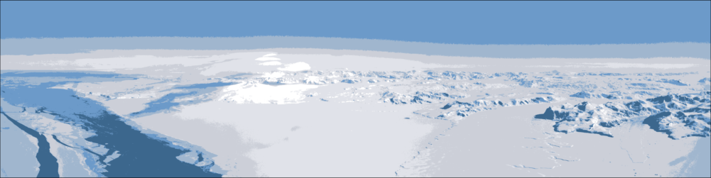
Now we can repeat the clustering and recoloring process to preview the new
palettized image, taking care to remember that the extra white pixel needs
to be removed from the image. I’ve also increased the cluster count by 1
so that \(n\) encodes the number of free color palette items in the fit.
km = kmeans(channelview(img_wwhite), n + 1; weights=w_wwhite,
            init=floor.(Int, range(1, length(img_wwhite), length=n+1)))
palette_wwhite = colorview(RGB{Float64}, km.centers)
rc_pix_wwhite = palette_wwhite[assignments(km)[1:end-1]]
recolored_wwhite = reshape(rc_pix_wwhite, size(img))

display(palette_wwhite)
display(recolored_wwhite)

Now adding in the weighted functionality into the palettize function
as an optional keyword argument,
function palettize(::Type{T}, imgin, n; seed=1111,
                   inc::Union{Nothing,Vector{<:Color}}=nothing) where {T<:Color}
    @assert isconcretetype(T)
    img = convert.(T, vec(imgin))
    nimg = length(img)

    if inc === nothing
        ninc = 0
        weights = nothing
    else
        ninc = length(inc)
        wn = one(float(eltype(T))) / (1 + ninc)
        weights = fill(wn / nimg, nimg)
        append!(weights, fill(wn, ninc))
        append!(img, inc)
    end

    km = kmeans(channelview(img), n + ninc, weights = weights,
        init = floor.(Int, range(1, nimg, length=n+ninc)))

    pal = collect(colorview(T, km.centers));
    idximg = pal[assignments(km)[1:(end-ninc)]]
    permute!(pal, sortperm(counts(km), rev=true))

    return (; palette=pal, idximg=reshape(idximg, size(imgin)))
end
palettize (generic function with 1 method)
palette_wwhite, recolored_wwhite =
    palettize(RGB{Float64}, img, 5, inc = [colorant"white"]);

display(palette_wwhite)
display(recolored_wwhite)


For a monochromatic palette like this one, it might be preferable to
sort the colors by brightness, which the Colors.jl makes very simple
by supporting a variety of colorspace transformations. To sort on
brightness, the Hue-Saturation-Lightness (HSL) colorspace will
work, and then we can print the hexadecimal color palette in CSS to make
direct importing to a website:
function colorsort_lightness(colors)
    c = HSL.(colors)
    L = view(channelview(c), 3, :)
    return colors[sortperm(L)]
end

display(colorsort_lightness(palette_wwhite))

println(":root {")
foreach(enumerate(colorsort_lightness(palette_wwhite))) do (i, c)
    println("    --header-palette-$i: #$(hex(c));")
end
println("}")

:root {
    --header-palette-1: #3C678D;
    --header-palette-2: #6C9AC9;
    --header-palette-3: #A0B6CE;
    --header-palette-4: #CCCFD8;
    --header-palette-5: #E0E2E8;
    --header-palette-6: #FFFFFF;
}