An algorithm for calculating special functions is no use if it has poor numerical accuracy and returns inaccurate or invalid answers. In this article I discuss the importance of using fused multiply-add (FMA) and a form of loop-unrolling to maintain numerical accuracy in calculating the associated Legendre polynomials to degrees and orders of order 1000 and greater.

Introduction¶

In this article we are going to explore a pair of simple yet important modifications to the existing legendre() implementation that are aimed solely at improving the numerical precision of the algorithm. The following two sections will each concentrate on one of the transformations, discussing in depth why the transformation is prudent, and the conclusion will tease a calculation I was performing which demonstrated the need for this careful attention to numerical accuracy.

As a reminder, the calculations proceed via the evaluation of the three following recurrence relations:

In particular, note that Eqn. $\ref{eqn:cus_rr_1term_lm}$ (the expression that steps along the matrix diagonal) is the precursor to the other two recursions. The implication is that any accumulated error in the first step propagates through the other two recurrences, so it is prudent to ensure the process starts with as much accuracy as possible.

There are essentially three parts to the recurrence — the previous term of the recurrence, the normalization-specific coefficient, and the factor of $\sqrt{1 - x^2}$. The only one we can meaningfully (and generically) effect is the square root factor, so let us consider that specifically. (Of course, the normalization-specific constants should also be calculated in a numerically accurate way, but since that’s specific to each case, we’ll just assume that has been done expertly here.)

In the following sections we will split the calculation of $y = \sqrt{1 - x^2}$ into two parts and analyze each of them independently. First, we’ll analyze and discuss the accuracy of calculating the inner component $y^2 = 1 - x^2$, and then the following section will concentrate on the impact of calculating the square root $y = \sqrt{y^2}$.

Fused Multiply-Add (FMA) in two-term diagonal recurrence¶

If you recall your algebra well, it should be immediately obvious that the polynomial $1 - x^2$ can be mathematically equivalently expressed as the product of factors $(1 - x)(1 + x)$. The slightly more generic case of any difference of squares $w^2 - x^2$ is a classic example from the well-known article “What Every Computer Scientist Should Know about Floating-Point Arithmetic”¹ by D. Goldberg that demonstrates that mathematical equivalence does not mean the expression is numerically equivalent within a calculation using floating point numbers. In that article, it is stated that the factored product is generally preferred over the difference of squares because the latter suffers from catastrophic cancellation whereas the former has only benign cancellation.

We can demonstrate this numerically by defining functions for each of the two forms and evaluating the functions with both standard Float64 64-bit floating point numbers and with arbitrary-precision BigFloat numbers. (In this case, the default 256-bit precision of the BigFloat numbers is sufficient to quantify the rounding error in the 64-bit floats.)

f₁(x) = 1.0 - x^2
f₂(x) = (1.0 - x) * (1.0 + x)

Since the functions are even, we will analyze only half of the domain $x \in [0, 1]$ since the span $-1$ to $0$ will be a mirror reflection of the result on $0$ to $1$. We’ll take 1 million samples spaced uniformly² within the range and calculate a reference answer $y’ = 1 - x^2$ at BigFloat precision. Then because we care about the fractional error and not the absolute magnitude — that is to say, a difference of 1 compared to 1 billion is just as significant a difference of $10^{-9}$ compared to $1$ — the difference will be normalized by $\varepsilon$, which is the corresponding size of the ulp³ (or “unit in last place”) appropriate for the result.

x  = collect(range(0.0, 1.0, length=1_000_001))
y′ = @. big(1.0) - big(x)^2
ε  = @. eps(Float64(y′))

ulperr(y) = @. Float64((y - y′) / ε)

Now we can calculate the maximum error for both f₁‌${} = 1 - x^2$ and f₂‌${} = (1-x)(1+x)$:

println("max err   1-x^2    = ", maximum(ulperr(f₁.(x))))
println("max err (1-x)(1+x) = ", maximum(ulperr(f₂.(x))))

max err   1-x^2    = 52233.570617393154
max err (1-x)(1+x) = 1.4976462110125

In agreement with the Goldberg article, the first form has a worst-case scenario which has much greater loss of precision in the final result. The simple maximum, though, is not very informative — if only a single pathelogical case is orders of magnitude worse, than the maximum is not a good representation of the behavior across the entire domain of interest.

Therefore, it’ll be more useful to plot the error in ulps for every sample. With one million points, no single marker or line segment will be visible; instead we’ll be looking at what are essentially shaded regions that envelope all answers within some span of the domain (with the span being implicitly defined by the pixel resolution of our plot).

using PyPlot, Printf

function summary_plot(fns, labels)
    for (fn,lbl) in zip(fns, labels)
        δ = ulperr(fn.(x))
        maxδ = maximum(abs, δ)
        plot(x, δ; linewidth=0.5, alpha=0.5,
            label = @sprintf("%s :: max err = %0.2f ulps", lbl, maxδ))
    end
    legend()
    xlabel(raw"$x$"); ylabel("ulps")
    ylim(-10, 10)
end

summary_plot((f₁, f₂), (raw"$1 - x^2$", raw"$(1-x)(1+x)$"))

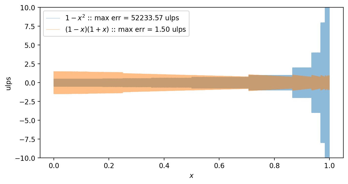
What we find is that the first form actually loses less precision than the second for about 75% of the domain (from $x = 0$ to about $0.75$), but as $x$ approaches $1$ it rapidly degrades in precision. This is precisely the catastrophic cancellation mentioned earlier.

In contrast, the second form is bounded across the entire domain, seemingly with no point having an error greater than 1.5 ulps. It is generally less precise for small values of $x$ but avoids the catastrophic cancellation as $x$ approaches 1.

The process of catastrophic cancellation can be shown through a simple example. Take the value $c = 1 - 2^{-30} \approx 0.9999999990686774$ and square it:

A standard double (64-bit) floating point value has only 51 base-2 digits of precision, so the small factor of $2^{-60}$ is truncated away and the result is rounded to $1 - 2^{-29}$. Now subtracting the quantity from 1 gives the result that $1 - c^2$ is $2^{-29}$:

c = 1 - 2^-30
1 - c^2 == 2^-29

true

Mathematically, this seems perverse because we can easily see that the two factors of $1$ cancel, so that

which spans only 31 powers of two and is well within the 51 orders representable by a double float. The relative error between the value $2^{-29}$ and $2^{-29}+2^{-60}$ is roughly 4 million ulps, which is certainly a catastrophic loss of precision!

This problem of intermediate rounding has long been recognized in numerical computing, and many mathematical transformations have been developed (like using the factored form $(1-x)(1+x)$) to maintain precision in calculations.

Thankfully for us, though, the operation $1 - x^2$ is a specific form of the more general $a \cdot b + c$, and that generic form is so crucial to a wide variety of algorithms that special “fused multiply-add” (FMA) functions have long been available that perform the computation at extended precision and only round the result once. Delaying the rounding of the squared term until after adding (or subtracting) in this case is exactly what is required to eliminate the common $1$ in the expression and collapse the range of digits to a span which does fit within a standard double float.

Adding the FMA calculation to our toolbox and comparing to the previous two cases:

f₃(x) = fma(-x, x, 1.0) # == (-x)*x + 1
summary_plot((f₁, f₂, f₃), (raw"$1 - x^2$", raw"$(1-x)(1+x)$", raw"fma(-x*x + 1.0)"))

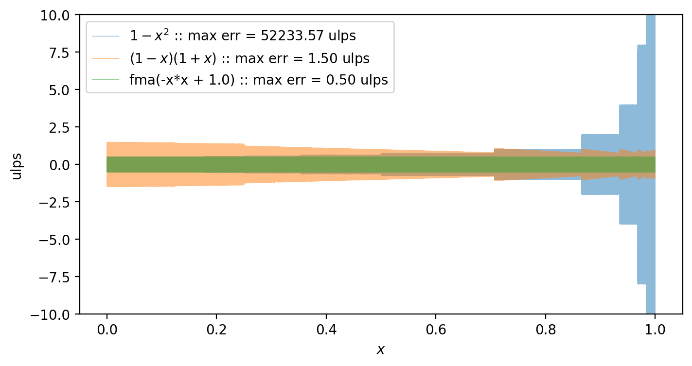
The FMA calculation is clearly the best option in terms of precision, with a maximum error of 0.5 ulps.

As of several years ago, the use of FMA instructions could be very expensive to utilize as it was implemented in software libraries rather than at the hardware level. At this point, though, a version of the FMA instruction has been supported⁴ in both Intel and AMD processors since circa 2011–2014 (and even more recently in many mobile (ARM) processors or GPUs as well). In the context of scientific computing, we can thankfully now reasonable assume the FMA instructions will be performed in hardware, so we have no reason not to improve the numerical precision of the Legendre polynomials by exploiting the FMA.

Pairwise unrolling the diagonal recurrence¶

The second improvement we can make is to simply recognize that the best way to preserve numerical accuracy in a calculation is to not do a calculation in the first place. Consider the first two iterations along the diagonal, given the initial condition $p_0^0$:

We have just established a way to accurately calculate $1 - x^2$, but the first iteration requires the square root of the quantity which will necessarily incur some more numerical rounding. The second iteration would benefit from just using the FMA quantity directly, but as the naive iteration proceeds, it is instead a square of the square-root quantity. We can easily show the extra error incurred by unnecessarily squaring a square root with the same summary plot used in the previous section:

r₁(x) = sqrt(f₃(x))^2
summary_plot((f₃, r₁), (raw"$1-x^2$", raw"$(\sqrt{1-x^2})^2$"))

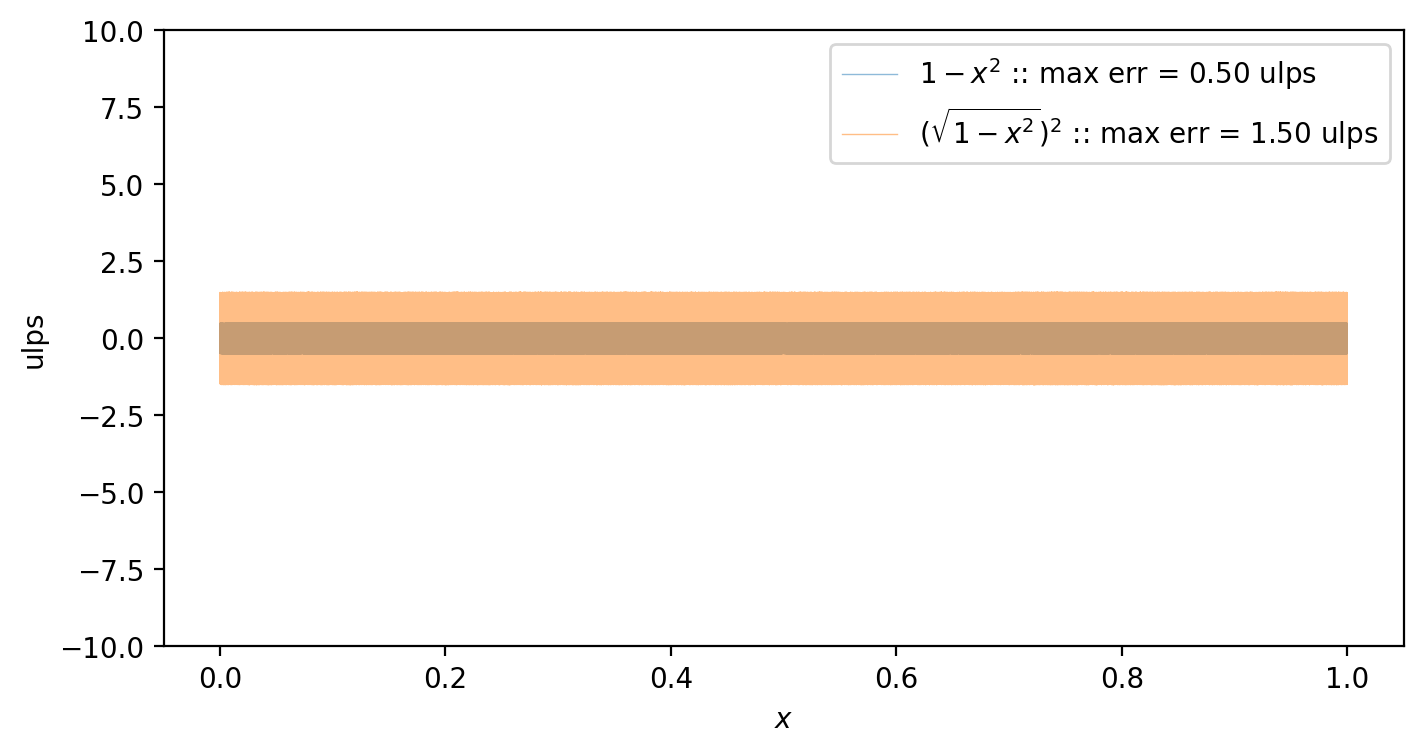
In general, a round-trip incurs one extra ulp of error across the domain. This error is then carried forward and amplified through the recurrence since each step builds upon the last.

A simple transform that can be made is to observe that the first two iterations are just a particular case of a more general pattern — odd degrees require one factor of $\sqrt{1 - x^2}$ in the product while even degrees can be written completely in terms of $1 - x^2$. Therefore, let us rewrite the recurrence relation Eqn. $\ref{eqn:cus_rr_1term_lm}$ as

Before modifying the legendre() implementation, let us first explore incrementally how each of the FMA and pairwise-unrolling of the diagonal recurrence impacts the numerical precision. Ignoring the normalization-specific coefficient factor (i.e. letting $\mu_\ell = 1$) and assuming $p_0^0 = 1$, then the recurrence relation simplifies directly to \begin{align*} p_\ell^\ell(x) = \left(1 - x^2 \right)^{\ell/2} \end{align*} We calculate this expression explicitly at extended precision for a 10,000 values of $x \in [0,1]$ and for all $0 < \ell \le 500$ to generate a matrix of values with 5 million entries.

Then at standard Float64 precision, we’ll calculate the recurrence (not as a direct power) for three cases:

1. The baseline case that lacks even the FMA improvement discussed above.
2. A version which introduces the FMA calculation of $1 - x^2$ to case 1.
3. A final version which further introduces on top of case 2 the pairwise loop iteration.

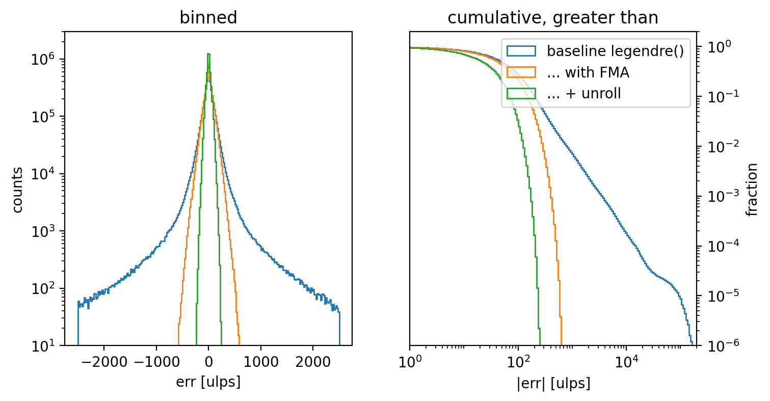
The matrices are very large, so we summarize them by histogramming the error of each version with respect the reference calculation.

The left panel of the plot below shows the binned histograms for the three cases on a horizontal axis that ranges up to 2500 ulps of error in either direction from the reference value. It is immediately obvious that the baseline case (blue line) has very long tails toward high error. To see the significance of that tail more clearly, the right panel of the figure instead plots the cumulative counts of (absolute) error values greater than or equal to a given error threshold on a logarithmic horizontal axis. The tail of this distribution reaches to nearly $2 \times 10^{5}$ ulps, and about 1% of all values have an error of about 700 ulps or greater.

When the naive calculation of $1 - x^2$ is replaced with the equivalent FMA calculation, the histogram (orange line) tightens considerably toward zero error. In fact, all terms have less than 700 ulps of error, so this change alone eliminates the long tails of the baseline version.

Finally, adding in the pairwise loop iteration as well further reduces the error, with the width of the histogram being about half of the FMA-only case.

lmax = 500 # even so that m÷2 is even as well
X  = collect(range(0.0, 1.0, length=10_001))

# The reference case
Y′ = @. sqrt((1 - big(X)^2)^(1:lmax)')
E  = @. eps(Float64(Y′))
ulperr2(Y) = Float64.((Y - Y′) ./ E)

# Case 1 -- baseline
Y₀ = zeros(length(X), lmax)
@. Y₀[:,1] = sqrt(1.0 - X^2)
for ii in 2:lmax
    @. Y₀[:,ii] = Y₀[:,ii-1] * Y₀[:,1]
end

# Case 2 -- with FMA
Y₁ = zeros(length(X), lmax)
@. Y₁[:,1] = sqrt(fma(-X, X, 1.0))
@inbounds for ii in 2:lmax
    @. Y₁[:,ii] = Y₁[:,ii-1] * Y₁[:,1]
end

# Case 3 -- + unroll
Y₂ = zeros(length(X), lmax)
@. Y₂[:,2] = fma(-X, X, 1.0)
@. Y₂[:,1] = sqrt(Y₂[:,2])
@inbounds for ii in 4:2:lmax
    @. Y₂[:,ii-1] = Y₂[:,ii-2] * Y₂[:,1]
    @. Y₂[:,ii]   = Y₂[:,ii-2] * Y₂[:,2]
end

# Plot generation
function summary_plot2d(Ys, labels)
    binslin = range(-2500, 2500, length=251)
    binslog = 10 .^ range(-1, 6, length=250)
    fig, axs = subplots(1, 2)
    for Y in Ys
        Δ = vec(ulperr2(Y))
        axs[1].hist(Δ, binslin; histtype=:step)
        axs[2].hist(abs.(Δ), binslog; histtype=:step, density=true, cumulative=-1)
    end
    axs[1].set(
        xlabel = "err [ulps]",
        yscale = "log", ylim = (10, 3e6), ylabel = "counts",
        title = "binned")
    axs[2].yaxis.set_label_position("right"); axs[2].yaxis.tick_right()
    axs[2].set(
        xscale = "log", xlim = (1, 2e5), xlabel = "|err| [ulps]",
        yscale = "log", ylim = (1e-6, 2), ylabel = "fraction",
        title = "cumulative, greater than")
    axs[2].legend(labels)
    return (fig, axs)
end

summary_plot2d((Y₀, Y₁, Y₂), ["baseline legendre()", "... with FMA", "... + unroll"])

Note that there are two reasons for not unrolling the iteration further. First, this investigation case was simplified by assuming $\mu_\ell = 1$, but in general the coefficient varies as a function of $\ell$; there is an implicit coefficient $\Pi_{\ell=1}^{\ell_\mathrm{max}} \mu_\ell$ that we were able to simplify away that would require keeping track of for a general normalization. Furthermore, direct calculation of $\left(1-x^2\right)^{\ell/2}$ with double floats actually results in an error distribution which is almost identical to the FMA+unrolled case, so there is very little motivation to further complicate the calculation.

Legendre calculation with FMA and pairwise unrolling¶

Let us finally update the legendre() implementation to take advantage of both the enhancements we have enumerated here. (The definitions of normalization trait types and property functions are unchanged from the previous post, so there are omitted here for brevity.)

The changes are straight-forward: we calculate the quantity $1 - x^2$ using an FMA instruction and store that as the value $y^2$. The iteration along the diagonal proceeds in steps of two where we employ only the even case of Eqn. $\ref{eqn:cus_rr_1term_lm_unroll}$ up to the last even integer less than or equal to the target $m$. Only if the target $m$ is odd does the function take a single step using the odd case of Eqn. $\ref{eqn:cus_rr_1term_lm_unroll}$ and the square root factor $y^1 = \sqrt{y^2}$.

The rest of the function to iterate through higher degrees $\ell$ off the diagonal is unchanged thereafter.

function legendre(norm, ℓ, m, x)
    P = convert(typeof(x), initcond(norm))
    ℓ == 0 && m == 0 && return P

    # Use recurrence relation 1 to increase to the target m
    y² = fma(-x, x, one(x))
    meven = 2 * (m ÷ 2)
    for m′ in 2:2:meven
        μ₁ = coeff_μ(norm, m′ - 1)
        μ₂ = coeff_μ(norm, m′)
        P = μ₁ * μ₂ * y² * P
    end
    if meven < m
        y¹ = sqrt(y²)
        μ₁ = coeff_μ(norm, m)
        P = -μ₁ * y¹ * P
    end
    ℓ == m && return P

    # Setup for 2-term recurrence, using recurrence relation 2 to set
    # Pmin1
    ν = coeff_ν(norm, m + 1)
    Pmin2 = P
    Pmin1 = ν * x * Pmin2
    ℓ == m+1 && return Pmin1

    # Use recurrence relation 3
    for ℓ′ in m+2:ℓ
        α = coeff_α(norm, ℓ′, m)
        β = coeff_β(norm, ℓ′, m)
        P = α * x * Pmin1 - β * Pmin2
        Pmin2, Pmin1 = Pmin1, P
    end

    return P
end

 function legendre(norm, ℓ, m, x)
     P = convert(typeof(x), initcond(norm))
     ℓ == 0 && m == 0 && return P
 
     # Use recurrence relation 1 to increase to the target m
-    y = sqrt(one(x) - x^2)
-    for m′ in 1:m
-        μ = coeff_μ(norm, m′)
-        P = -μ * y * P
+    y² = fma(-x, x, one(x))
+    meven = 2 * (m ÷ 2)
+    for m′ in 2:2:meven
+        μ₁ = coeff_μ(norm, m′ - 1)
+        μ₂ = coeff_μ(norm, m′)
+        P = μ₁ * μ₂ * y² * P
+    end
+    if meven < m
+        y¹ = sqrt(y²)
+        μ₁ = coeff_μ(norm, m)
+        P = -μ₁ * y¹ * P
     end
     ℓ == m && return P
 
     # Setup for 2-term recurrence, using recurrence relation 2 to set
     # Pmin1
     ν = coeff_ν(norm, m + 1)
     Pmin2 = P
     Pmin1 = ν * x * Pmin2
     ℓ == m+1 && return Pmin1
 
     # Use recurrence relation 3
     for ℓ′ in m+2:ℓ
         α = coeff_α(norm, ℓ′, m)
         β = coeff_β(norm, ℓ′, m)
         P = α * x * Pmin1 - β * Pmin2
         Pmin2, Pmin1 = Pmin1, P
     end
 
     return P
 end

All of this effort spent to study the numerical accuracy of the diagonal recurrence relation is not merely an interesting academic exercise. I was driven to investigate this path through a concrete example where the loss of precision led to non-physical results in a calculation.

Without going into greater detail (which may appear in a future article), I was interested in calculating a quantity that included a term similar to:

where $\lambda_\ell^m(x)$ is the spherical-harmoinc normalization of the Legendre polynomials. The value of $Q_\ell$ was well-behaved at low-$\ell$, but suddenly diverged in an unexpected way after some critical point. After some investigation, I concluded that the cause was specifically the Legendre term, and I narrowed down a representative case to the following slice of the matrix over degrees and orders for a fixed $\ell$:

function example_use(legendre_fn)
    # Constants for a particular use of legendre functions
    lmax = 2125
    θlim = deg2rad.((147.375, 147.875))
    xs = range(cos.(θlim)..., length=100)
    # λlm_lmax^m(x) for m ∈ 0:lmax
    Λ = [legendre_fn(SphereNorm(), lmax, m, x) for x in xs, m in 0:lmax]
    # "integrated" over all xs in a small range
    Λint = step(xs) .* dropdims(sum(Λ, dims=1), dims=1)
    return Λint
end

# legendre_prev() is the legendre() implementation taken from the end of Part III
plot(example_use(legendre_prev), linewidth=0.5, label="previous legendre()")
plot(example_use(legendre), linewidth=0.5, label="legendre() with FMA+unroll")
title("Example use of Legendre functions")
legend()
xlabel(raw"$m$")
ylabel(raw"$\approx\int_{-0.8422}^{-0.8469}\lambda_{2125}^m(x)\,dx$")

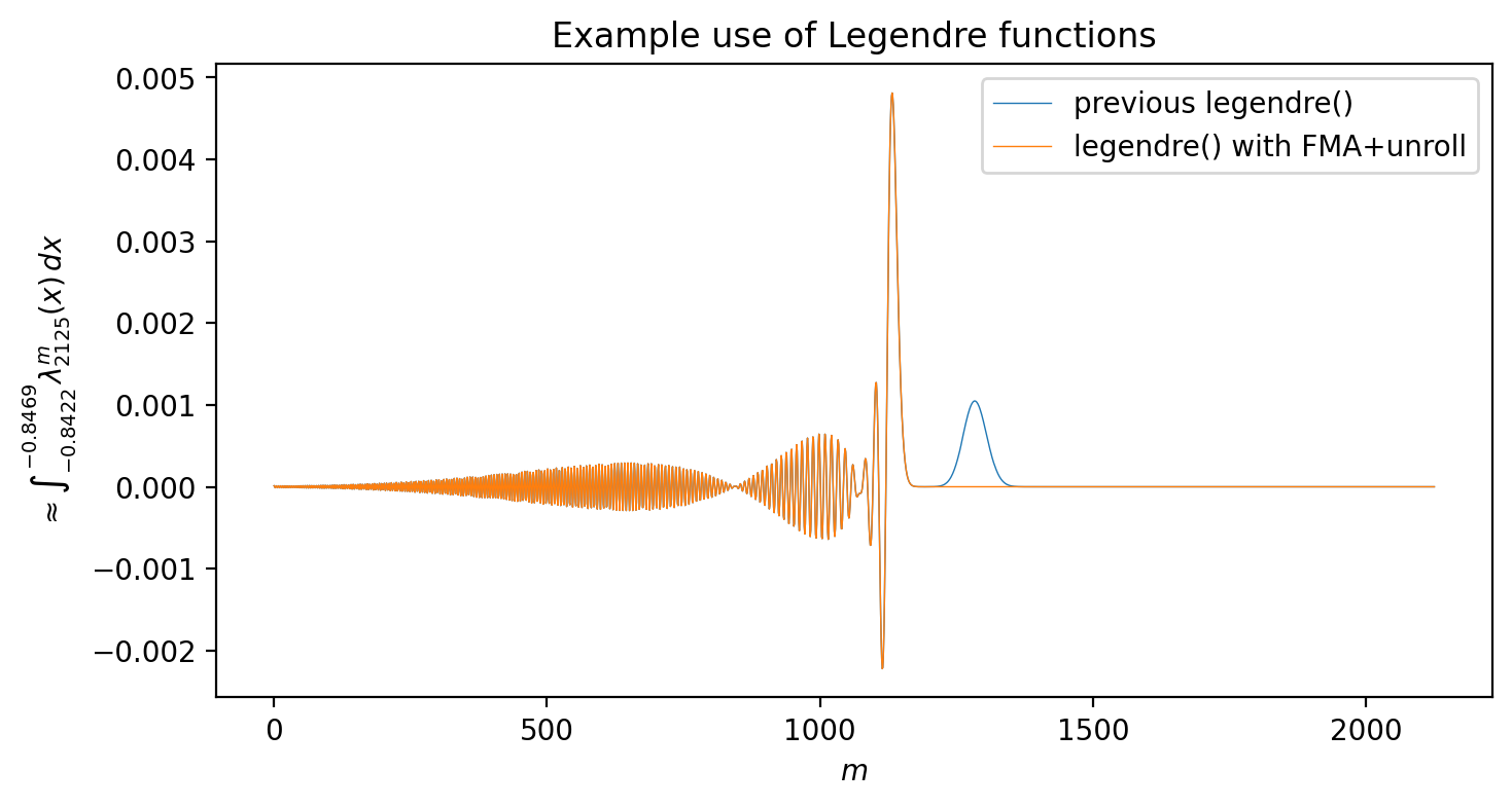
Without the improvements explored in this posting, the integral for fixed degree $\ell$ has a brief period of aberrant growth (blue line near $m = 1250$) before the normalization suppresses the function. The disturbance continues to grow with higher degrees, so the average over all orders $m$ was dominated by this numerical instability and the desired quantity $Q_\ell$ had an unwanted divergence.

The orange line instead shows the same quantity calculated using the improved implementation that makes use of the FMA and partially-unrolled recurrence enhancements. The function is very similar everywhere except around $m = 1250$ where the hump disappears. When extended to all higher degrees as well, these changes solved the problems with calculating the quantity $Q_\ell$ and allowed me to complete my desired task.